What Determines the Spread Between Brent and WTI?

Introduction

Crude oil is one of the most important commodities in global financial markets, and two benchmarks dominate pricing: West Texas Intermediate (WTI) and Brent crude oil. WTI is primarily used as a benchmark in the United States, while Brent serves as the global benchmark, particularly in Europe and international markets. Although these two benchmarks generally move closely together due to shared macroeconomic drivers, their price spread (Brent − WTI) can vary significantly over time.

Understanding the dynamics of this spread is important for several reasons. First, it reflects regional supply-demand imbalances, transportation constraints, and geopolitical factors. Second, it is widely used in statistical arbitrage strategies, where traders exploit temporary divergences between the two benchmarks. Finally, studying volatility and correlation between Brent and WTI can provide insight into broader market stress and regime changes.

The objective of this project is to conduct an exploratory data analysis (EDA) of Brent and WTI crude oil prices using historical data obtained from the Federal Reserve Economic Data (FRED) API. Specifically, my analysis aims to (1) examine how crude oil prices have evolved over time, (2) analyze the behavior of the Brent–WTI spread, (3) investigate volatility patterns and extreme events, (4) evaluate the correlation between the two benchmarks, and (5) identify seasonal patterns in returns.

Methodology

The data used in this analysis was obtained from the FRED API, which provides daily spot prices for both WTI and Brent crude oil. The specific series used were DCOILWTICO for WTI and DCOILBRENTEU for Brent, both measured in U.S. dollars per barrel. The dataset spans from January 2000 through early 2026, providing over two decades of observations.

Before performing any analysis, the data required several preprocessing steps. First, the raw values were converted into numeric format, with any non-numeric entries were turned into missing values. Dates were parsed into a standard datetime format to allow for proper time series analysis. The two datasets were then merged on the date column to align observations across both benchmarks.

Because financial time series often contain gaps due to weekends and holidays, missing values were handled using forward filling. This approach carries the last observed price forward, which is reasonable in this context because markets are closed during non-trading days and prices typically remain unchanged during those periods.

To better understand the relationship between Brent and WTI, several derived variables were constructed. The most important of these is the spread, defined as the difference between Brent and WTI prices. This variable captures the divergence between the two benchmarks and serves as the central focus of the analysis.

Daily returns were also calculated to measure relative price changes over time. Both simple returns and log returns were computed. I included the log returns for some more financial rigor and to more accurately stabilize large price movements. Log returns by nature are additive over time which makes them useful for time series models and specifically for volatility calculations. In addition, rolling volatility was calculated using a 20-day window, allowing for the examination of how market risk evolves over time.

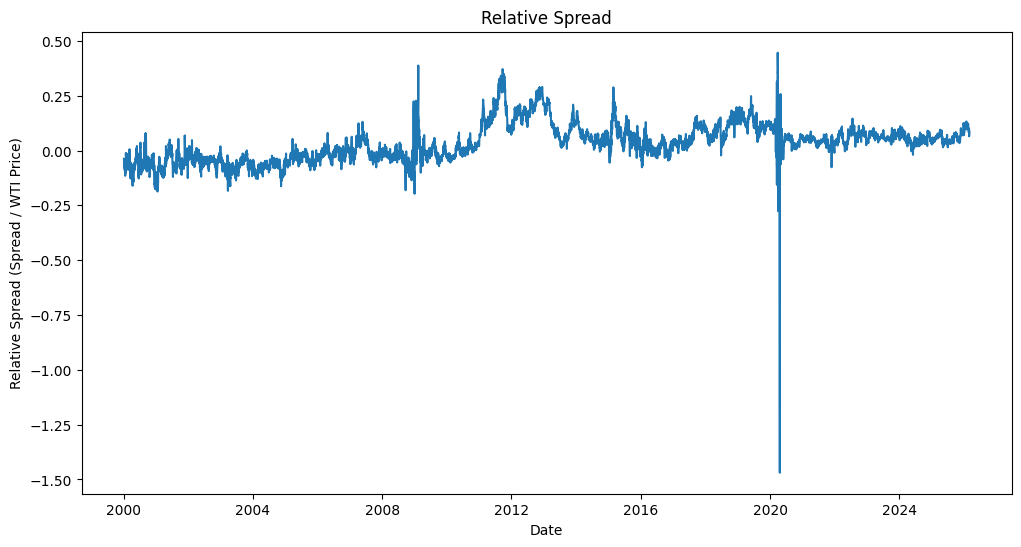
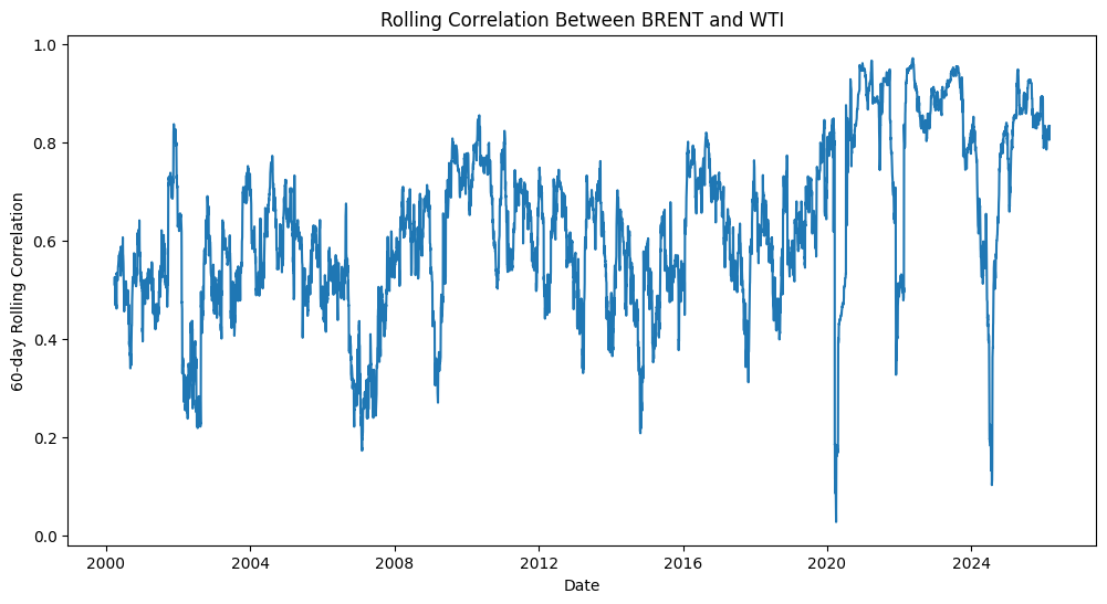
To assess the relationship between the two benchmarks, a 60-day rolling correlation was computed based on returns. This provides a dynamic view of how closely Brent and WTI move together across different market conditions. A relative spread measure was also introduced by scaling the spread by the WTI price, making it easier to compare spread magnitudes across different price levels.

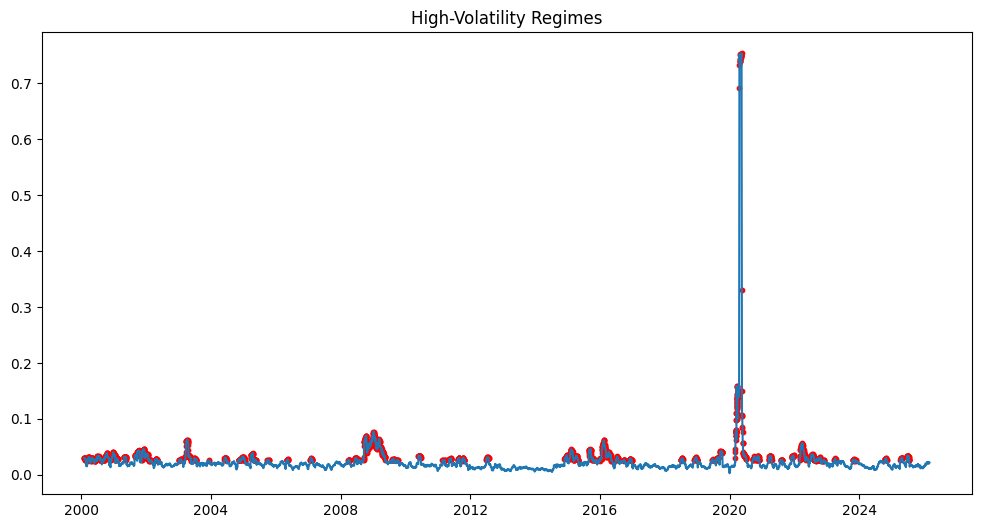
Finally, a volatility regime indicator was created by identifying periods where rolling volatility exceeds the 75th percentile. This allows for the classification of high-volatility environments and helps highlight periods of market stress.

The limitations of my project also need to be mentioned. Firstly, FRED provides spot price data, not futures curves, so it reflects current market conditions rather than forward-looking expectations or risk premiums. There’s no adjustment for inflation or currency effects. Also, this is still mostly descriptive work (no formal causal modeling). I’m only using spot prices, and forward-filling non-trading days is a reasonable but imperfect choice. There’s also only so much you can separate storage effects, transport issues, and geopolitics using benchmark prices alone. All of these are real constraints on how deep the conclusions can go.

Exploratory Analysis

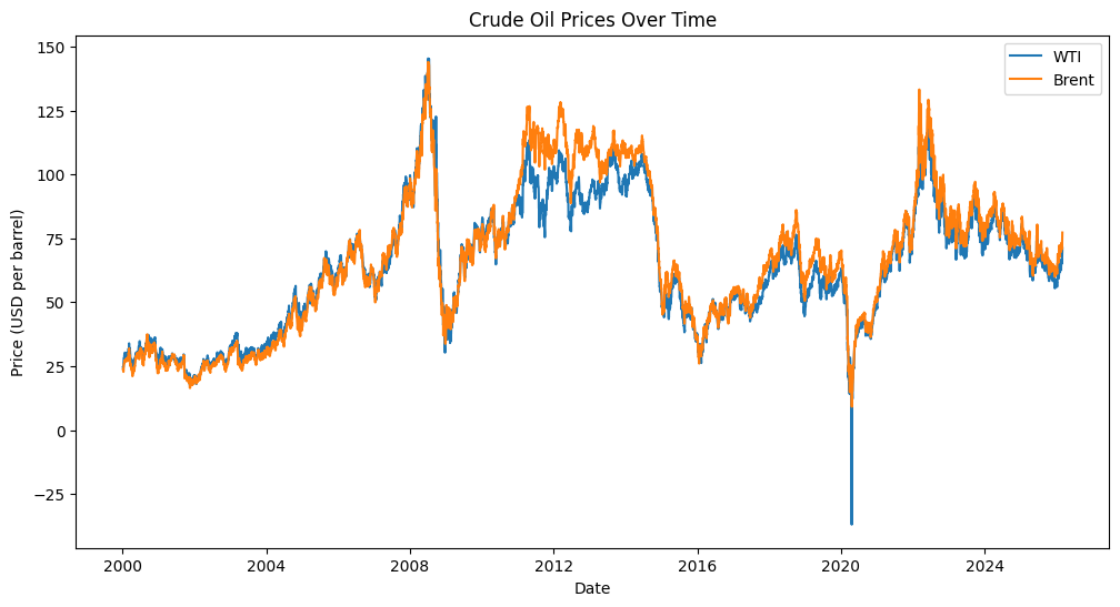
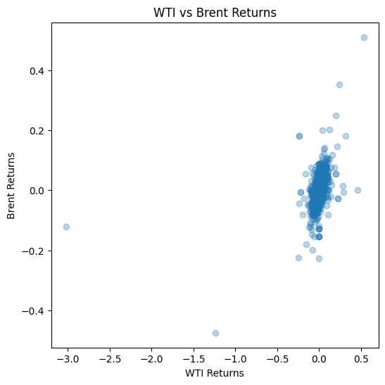
The time series of crude oil prices reveals several important patterns. Brent and WTI prices generally track each other closely, confirming that they are driven by similar underlying economic forces. However, there are notable periods where prices diverge or exhibit extreme behavior. For example, both benchmarks experienced a sharp rise leading up to the 2008 financial crisis, followed by a dramatic collapse. Another significant disruption occurred in 2020 during the COVID-19 pandemic, when demand shocks and storage constraints caused unprecedented market conditions. Notably, WTI prices briefly turned negative during this period, reflecting the cost of storage exceeding the value of the commodity itself. The transportation sector drives demand for refined petroleum products (e.g., gasoline, diesel, jet fuel), which dropped during the lockdown. I highlight COVID as it was a unique point in history during which humans demanded 30% less oil/gas. Brent is seaborn so I suspect storage wasn’t as difficult as with WTI (i.e Brent is stored and shipped via coastal terminals and tankers whereas WTI is landlocked at Cushing, Oklahoma, which made storage constraints far worse during the 2020 crash).

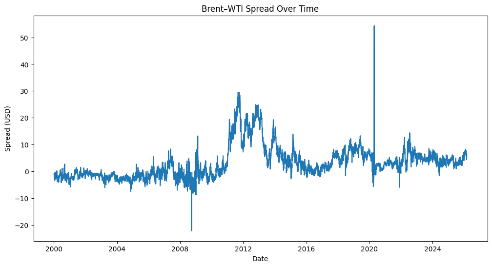
The Brent–WTI spread provides further insight into these dynamics. For most of the sample period, the spread remains relatively small, suggesting that the two benchmarks are closely linked. However, there are several episodes where the spread widens significantly. One such period occurs between 2011 and 2013, likely driven by infrastructure bottlenecks in the United States that limited the ability to transport oil efficiently.

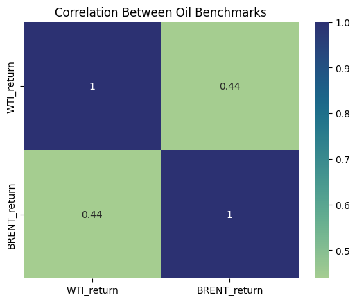
The rolling correlation analysis reinforces this interpretation. While the correlation between Brent and WTI is generally high, it declines sharply during periods of market stress. This suggests that although the two benchmarks are typically driven by common factors, their relationship can weaken when markets experience structural shocks.

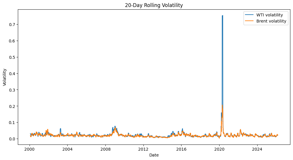
Volatility analysis reveals a similar pattern. For most of the sample period, volatility remains relatively low and stable. However, it increases dramatically during crisis periods, particularly in 2008 and 2020. These spikes illustrate the concept of “volatility clustering”, where periods of high volatility tend to be followed by additional high-volatility periods. Interestingly, WTI volatility tends to spike more sharply than Brent, most likely reflecting its greater exposure to localized factors such as storage and transportation constraints.

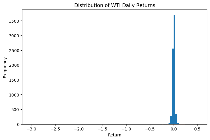
The distribution of daily returns further highlights the presence of extreme events. Most returns are concentrated near zero, indicating small day-to-day price changes. However, the distribution exhibits fat tails, meaning that large positive or negative returns occur more frequently than would be expected under a normal distribution. This is a common feature of financial data and has important implications for risk management.

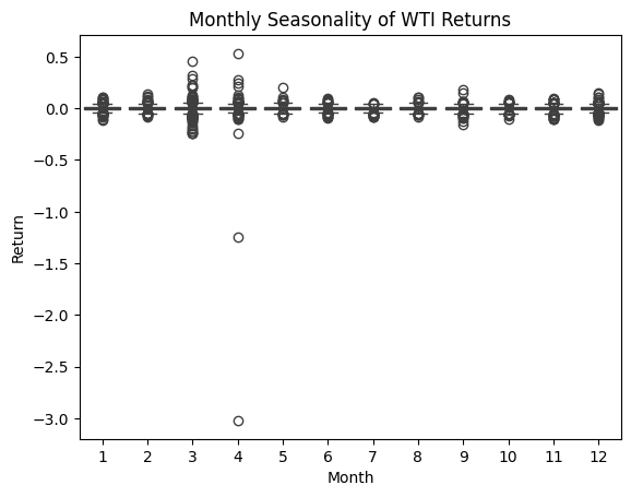
Seasonality analysis, based on grouping returns by month, suggests that there is no strong or consistent seasonal pattern in oil returns. While certain months exhibit more variability than others, these effects are relatively minor compared to the impact of major economic or geopolitical events.

Additionally, the identification of high-volatility regimes shows that periods of market stress are not isolated events but tend to cluster over time. This reinforces the idea that financial markets exhibit persistent periods of instability, rather than purely random fluctuations.

Conclusion

So how have crude prices changed over time? There is no one-way ticket, but it has largely been up and to the right—as one would expect—due to our increased demand for oil and gas over time. This is attributed to technological developments and globalization, all of which require fuel to be sustained.

Overall, my analysis reveals that Brent and WTI are highly interconnected but not perfectly aligned. Their prices generally move together, but temporary divergences can arise due to regional constraints, infrastructure limitations, or global shocks. The Brent–WTI spread is therefore best understood as an episodic phenomenon, rather than a persistent trend.

Volatility and correlation both play crucial roles in understanding this relationship. During stable periods, the two benchmarks exhibit high correlation and low volatility. In contrast, crisis periods are characterized by increased volatility and a breakdown in correlation, reflecting underlying market stress.

The COVID-19 pandemic stands out as the most extreme event in the dataset, producing unprecedented volatility and a temporary decoupling of prices. This highlights the importance of considering rare but impactful events when analyzing financial markets.

Motivation

During an interview, I mentioned that I have a background in commodities (I was an accounting intern at an oil company last summer, and my family is from an oil rich country). He asked me “wow...so what do you think about the spread between WTI and Brent?” I didn’t know how to answer and just said “Oh I mostly follow crude price action.” Which, in hindsight, is just about the stupidest answer I could have given...no really, it would have been better to just say “I don’t know.” Anyway, I thought I’d take this as an opportunity to formally figure out the answer to that one.